
One of my favorite conference talks of all time is Statistics Without the Agonizing Pain, by John Rauser, who was at that time head of data science at Pinterest. In this talk, he explains the statistical argument underpinning the Student’s t-Test in simple, approachable terms using an unforgettable example involving mosquitoes and beer. It’s about 15 minutes long, and well worth your time, if you haven’t watched it before.
After watching that video, I realized that—like most things—statistics is complex but ultimately straightforward once you understand the underlying ideas. The problem is that the modern approach to teaching statistics often gets in the way of that understanding. Historically, statistical methods were designed for a world where all computation had to be done by hand, so they were optimized to minimize calculation, not to maximize clarity or intuition. That design choice still has value today—efficient algorithms make modern statistical programs fast and practical. But we continue to teach statistics as if computation were still the bottleneck, even though we now all carry supercomputers in our pockets. Seen in that light, it’s obvious that the way we teach statistics has not kept up with the way we practice statistics.
To that end, I thought I’d write down some things I’ve learned about statistics over the years in a way that I hope is clearer than the average statistical textbook, mostly so I don’t forget them, but in the hopes that maybe they’ll be useful to others, too.
Probability Distributions
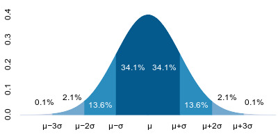
At the foundation of almost everything in both both frequentist and bayesian statistics is the idea of a probability distribution. A probability distribution is simply a description of how probability mass is spread across the possible values of a single variable. Visually, it can be thought of as a curve whose total area is equal to one. That curve might be narrow or wide, symmetric or skewed, with short tails or long ones, depending on how probability mass is concentrated.
The domain of a distribution matches the domain of the variable it describes. Categorical or integer-valued variables have discrete distributions, while real-valued variables have continuous distributions whose domain may be finite or infinite, depending on the variable. All of these characteristics describe how probability mass is arranged, but the defining feature is always the same: when you add up all the probability—by summing in the discrete case or integrating in the continuous case—you get exactly one.
Joint Probability Distributions
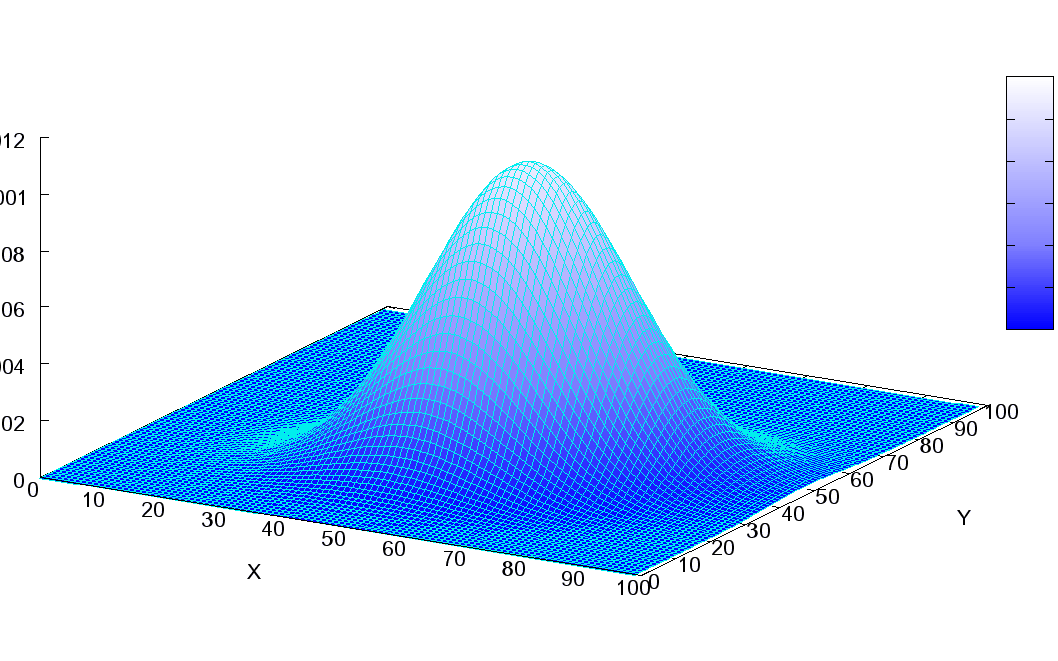
But what if you have more than one variable? You can think of a joint probability distribution as a plot of one probability distribution against another (or two, or three, and so on, for as many variables as you have).
A joint probability distribution of two variables X and Y is written as P(X, Y). The probability at a specific point (xi, yj) is written as p(.xi, yj)
Instead of assigning probability mass to individual values, it assigns probability mass to combinations of values from both single-variable distributions. Where a probability distribution gives a line, a joint probability distribution of two variables gives a surface, and three or more give a hypersurface.
For example, here is a visualization of a two-way multivariate normal distribution as a surface, from a three-quarter view:
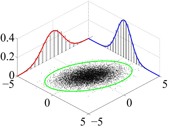
Here is another view of a similar multivariate normal distribution, now showing the individual normal distributions plus the joint distribution as a “dot map.” They both depict the same information.
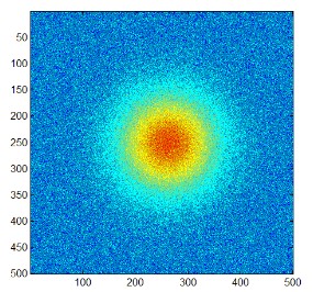
And another view of a similar distribution, this time from directly above, as a classical heat map, where probability values are depicted by color from low (blue) to high (red).
As with any probability distribution, the defining constraint is the same: when you add up all the probability under the resulting (hyper)surface —by summing in the discrete case or integrating in the continuous case—you get exactly one.
Conditional Probability Distributions
If joint probability distributions are plots of two (or three, or four, …) variables against each other, then conditional probability distributions are slices of those plots at a specific value of one (or more) of those variables.
A conditional probability distribution of two variables X and Y is written as P(Y | X) and is read “the probability of Y given X”. Crucially, this does not refer to a single distribution, but rather to a family of distributions: one for each value of X.
When we fix X to a specific value xi, we write P(Y | X = xi) and read “the probability of Y given X equals x sub i.” This represents a single, one-dimensional probability distribution over Y, obtained by slicing the joint distribution at X = xi and normalizing so that the total probability equals one.
This diagram shows “slices” P(X|Y=yi) of the conditional probability distribution P(X|Y) at various values for Y=yi.
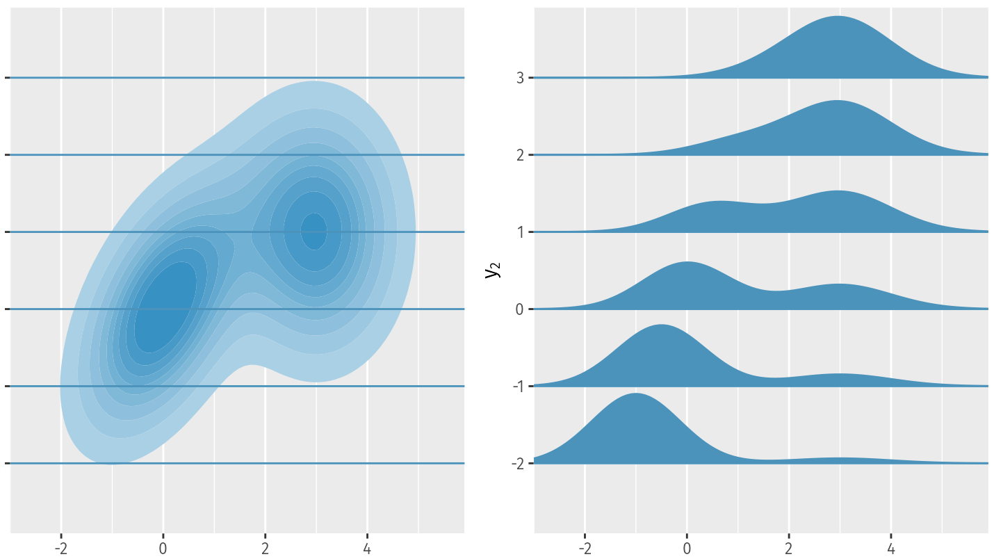
Again, as with any probability distribution, the defining constraint is the same: the sum of probability mass across the entire domain must add up to one.
Conditional vs Joint Probability Distribution Identities
Now that we understand that joint probability distributions are essentially “full plots” and conditional probability distributions are “slices” of those plots, this identity relationship between the two makes a lot more sense:
P(X, Y) = P(Y | X) * P(X)
Essentially, the probability at any point (xi, yj) is equal to the “slice” P(Y | X = xi) evaluated at yj times p(xi). This can be understood as a two-dimensional probability “lookup”.
Conclusion
Hopefully this helped simplify some of the basic concepts around probability distributions!