Fundamentals of Software Optimization Part II — Optimizing Wall Clock Performance

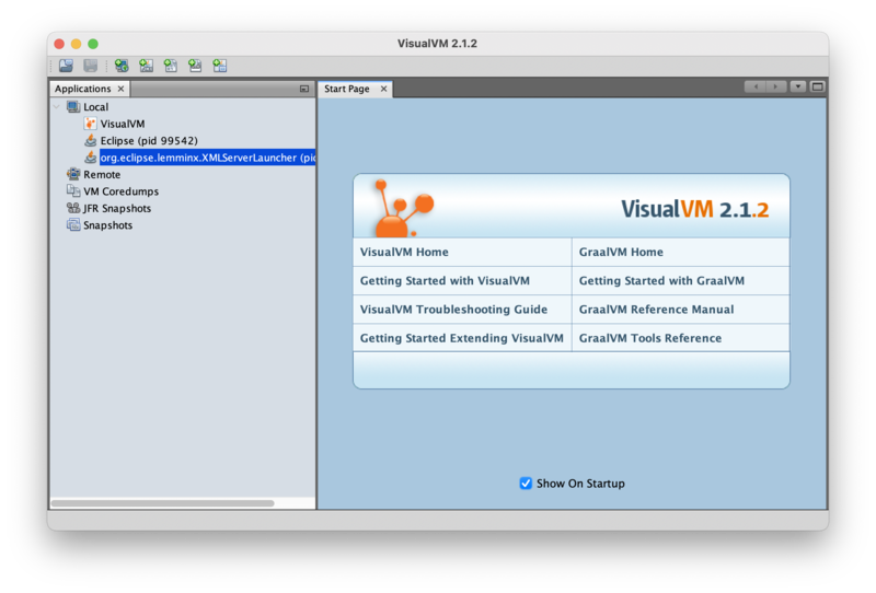
Meet VisualVM

The JVM has several good profilers. This series will use VisualVM, which is an excellent, user-friendly profiler for the JVM developed by the Java team. VisualVM has both sampling and instrumenting profilers. Because the focus of this post is optimizing wall-clock performance, only the sampling profiler will be used.

VisualVM can profile remote JVMs, but this series will profile locally for simplicity. The author has confirmed ahead of time that the results are directionally the same when profiling in the benchmark environment and locally. Users looking for instructions to profile the benchmark system remotely should find this documentation a good starting point.

VisualVM automatically detects programs running locally, so to start profiling the benchmark, simply run it. VisualVM should automatically detect two new running VMs: the “main” jar, which is the “parent” process; and the “ForkedMain” program, which is the actual running benchmark. Double click on the ForkedMain process in the left pane because that is the workload to be optimized. That should create an analysis tab for that JVM.

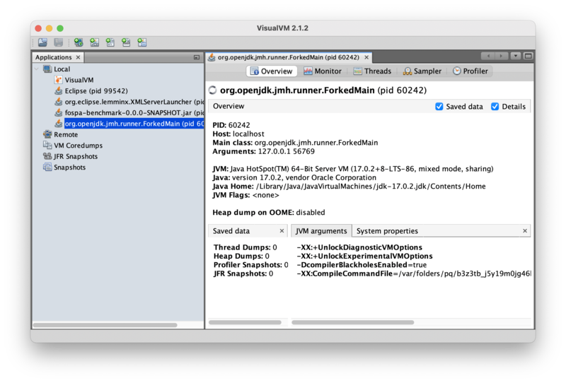
Note that if the program being profiled exits, then VisualVM automatically disconnects, and the analyst may need to restart their analysis on a new VM. It’s perfectly kosher to increase the number of iterations in the benchmark to reduce disconnects as long as the number gets changed back prior to any performance measurement.

The Optimization Workflow

The goal of software optimization is to improve program performance on some dimension(s). The focus of this post is wall clock performance, but the same process applies to all optimization:

1. Run a profiler to measure where the program is spending its resources (e.g., wall-clock time, allocations, memory, etc.) and identify “hot spots,” or small parts of the program that use a large amount of resources.
2. Find the biggest hot spot and make a change to improve program performance. Always focus on the biggest hot spot first because these improvements have the biggest potential for impact, by definition.
3. Measure performance with the change. If program performance did not improve, then roll back change and go back to step 3. Otherwise, continue.
4. Is the program fast enough? If so, optimization is complete! Otherwise, go back to step 1.

Essentially, find the biggest hot spot and fix it, over and over again, until the program is fast enough, at which point optimization is complete. (What is “fast enough” is generally a business decision, but as the introduction mentioned, this series is explicitly avoiding the discussion of business problems to focus on technical problems.)

An Example Wall Clock Optimization from Start to Finish

When optimizing for wall clock performance, sampling CPU utilization is always a good first step.

Collecting a CPU Performance Profile

Click on the “Sampler” button, and then click the “CPU” button. VisualVM should start collecting performance information:

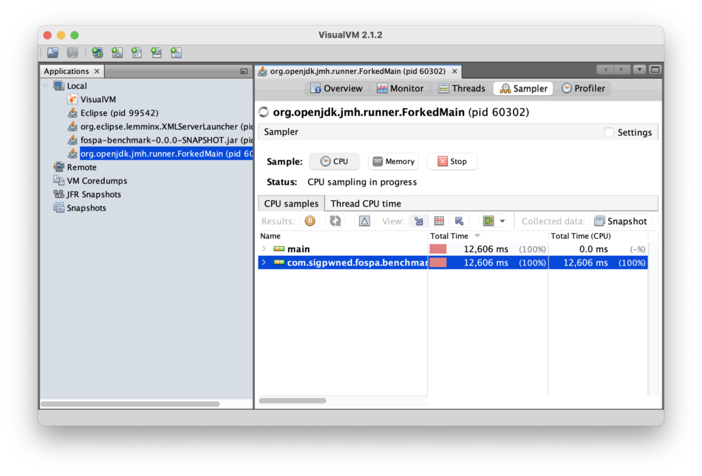
Clicking the stop button stops data collection. In general, 30 seconds is enough data to get a sense for “hot spots” that take a long time in a homogenous workload.

Looking for Hot Spots

Once data collection has been stopped, clicking the “Hot spots” button (between the two arrows, in the middle bar) will open a table that highlights the methods in which the program spends most of its time:

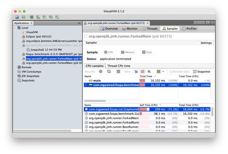
Immediately, the profiler can tell us that most program time is being spent in GraphemeMatcher.find(). This is not too surprising, since that’s more or less the whole benchmark! But the profiler zeroes in on this method immediately out of the box.

Note that the method’s “total time” is 16,004ms, but the “self time” is only 299ms. In other words, the program spent 16sec executing the GraphemeMatcher.find() method, but only 299ms in the GraphemeMatcher.find() method itself; the rest of that time was spent in methods that GraphemeMatcher.find() had called. Clicking into the jmh-worker thread drills into that thread to show the methods GraphemeMatcher.find() called where time is actually being spent:

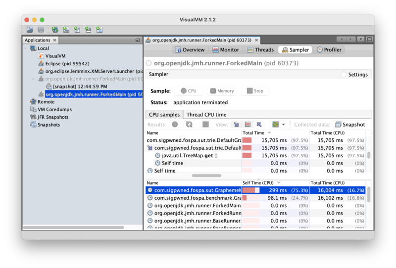
Drilling into the GraphemeMatcher.find() method reveals that 15,705ms of self time –or 98% of program time — is being spent in java.util.TreeMap.get(). That’s a hot spot!

Optimizing Code

Now that it’s clear where the program is spending it’s time, code optimization can begin. The offending DefaultGraphemeTrie source code is:

  private final Map<Integer, DefaultGraphemeTrie> children;
  private Grapheme grapheme;

  public DefaultGraphemeTrie() {
    this.children = new TreeMap<>();
  }

  @Override
  public DefaultGraphemeTrie getChild(int codePoint) {
    return children.get(codePoint);
  }

  private void put(int[] codePointSequence, Grapheme grapheme) {
    DefaultGraphemeTrie ti = this;
    for (int codePoint : codePointSequence)
      ti = ti.getOrCreateChild(codePoint);
    ti.setGrapheme(grapheme);
  }

  private DefaultGraphemeTrie getOrCreateChild(int codePoint) {
    DefaultGraphemeTrie result = children.get(codePoint);
    if (result == null) {
      result = new DefaultGraphemeTrie();
      children.put(codePoint, result);
    }
    return result;
  }

So DefaultGraphemeTrie is using a TreeMap to store trie children. The code does not appear to rely on the sorted nature of the underlying map, so it’s safe to drop in a more efficient implementation. What if the code were changed to use a HashMap instead? (Recall that a hash map is O(1) on reads, whereas a balanced tree map is O(log n) on reads.) Making that change, rebuilding the benchmark, and re-running the profiler produces this data:

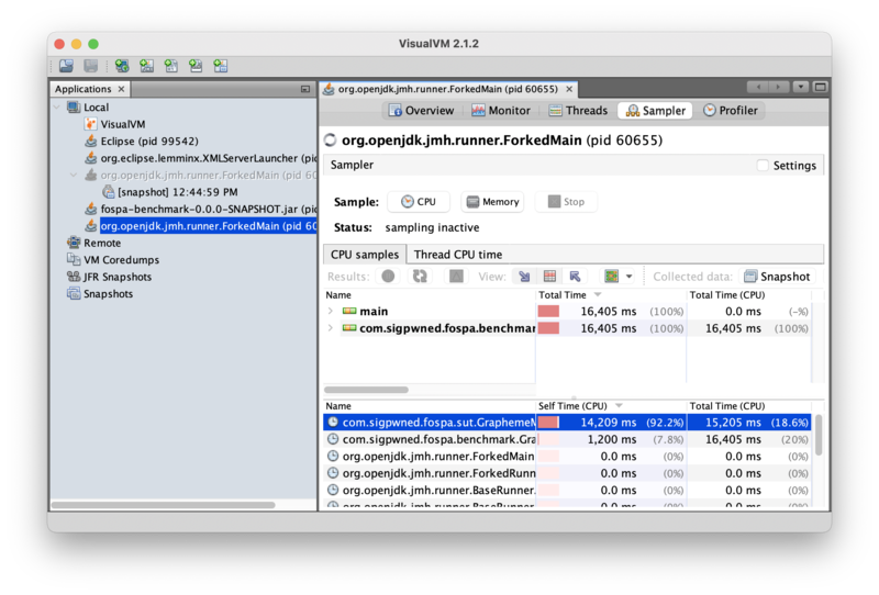
Self time for GraphemeMatcher.find() has increased from 1.87% of program time to 93.4%. That’s a huge change! So where the program used to spend most of its time in TreeMap.get(), it is now spending most of its time in GraphemeMatcher.find(). This should result in a substantial improvement to throughput because the program is now spending time doing useful work and instead of just retrieving trie children.

Benchmarking the Change

Recall the following baseline benchmark results from Part I:

Benchmark                         Mode  Cnt   Score   Error  Units
GraphemeMatcherBenchmark.tweets                                thrpt   15       19.383 ±     0.482   ops/s

It’s time to re-run the benchmark against the changed program to see if performance got better or worse. (Remember to use the proper EC2 environment!) The performance results for the updated benchmark are:

Result "com.sigpwned.fospa.benchmark.GraphemeMatcherBenchmark.tweets":
  53.416 ±(99.9%) 2.194 ops/s [Average]
  (min, avg, max) = (51.887, 53.416, 56.283), stdev = 2.052
  CI (99.9%): [51.222, 55.610] (assumes normal distribution)

The benchmark performance has been increased from a baseline of 19.322 MB/s to 53.416 MB/s, for a throughput improvement of 2.76x. Not bad!

Conclusion

This is the magic of a profiler: it allows an analyst to walk up to a running program they know nothing about, identify hot spots, and make meaningful performance improvements in a targeted fashion, often within hours. Optimization itself is generally straightforward, if not easy; in this (admittedly somewhat contrived) example, it was just changing one line of code! The hard part is knowing which lines to change. This is where the profiler shines.

Next Steps

Now that the program is running faster on wall-clock performance, we will look at memory allocation performance in Part III — Optimizing Memory Usage. See you there!