Fundamentals of Software Performance Analysis Part III — Optimizing Memory Allocation Performance

This is the third post in a three-post series covering the fundamentals of software performance analysis. You can find the introduction here. You can find Part II here. You can find the companion GitHub repository here.

Part II covered the process of using a profiler (VisualVM) to identify “hot spots” where programs spend time and then optimizing program code to improve program wall clock performance.

This post will cover the process of using a profiler to identify memory allocation hot spots and then optimizing program code to improve memory allocation performance. It might be useful to refer back to Part II if you need a refresher on how to use VisualVM or the optimization workflow.

An Example Memory Optimization From Start to Finish

Modern programming languages like Java support important “quality of life” features to make developers more productive, like automated memory management using a garbage collector. This laissez-faire approach to memory management is a huge win for development simplicity and velocity, but it also makes it easy to forget how much memory is being allocated. Reducing memory allocation is a good idea, especially in a data processing library like the benchmark workload, because high allocation may affect a downstream user’s performance.

When measuring memory usage, sampling memory utilization is always the first step. Kick off a benchmark run, and then connect to it using VisualVM. Click on the “Sampler” button, and then click the “Memory” button. VisualVM should start collecting memory performance information:

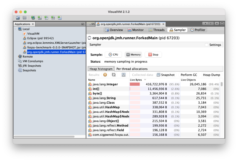
Most of the live dataset (95.6% by bytes, 99.4% by instance count) is instances of java.lang.Integer! If those instances are static data, like the GraphemeTrie loaded during benchmark initialization, then that does not affect memory allocation performance because they are simply the working set, but if these instances are being created during text processing, then there could be some allocation traffic to get back. Clicking on the delta button (the triangle next to the refresh button in the middle toolbar) will show how memory usage is changing in real time:

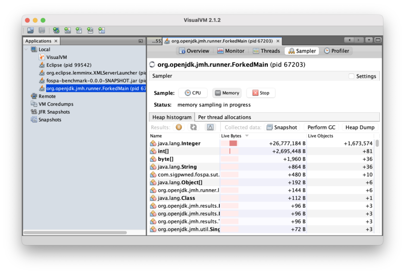
Integer instances are being created in real-time! Remember, the delta view shows changes in memory usage, so this data reveals that 1.67M instances of Integer occupying 26.7MB of heap space were allocated as the view is being updated.

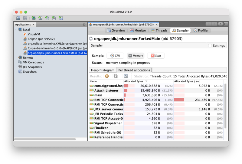
But the profiler is measuring the whole process, not just the benchmark thread. Perhaps the allocations are happening on another thread unrelated to the benchmark workload? Clicking the “Per-thread allocations” tab will answer that question:

The allocations are happening on the benchmark thread. And the thread is allocating a total of 760MB/sec, but only processing 53MB/sec! There is definitely room for improvement. But what code is allocating the Integer instances? Taking a heap dump of the running program may provide some guidance. Going back to the “Heap histogram” tab and clicking the “Heap Dump” button will show the heap dump summary screen:

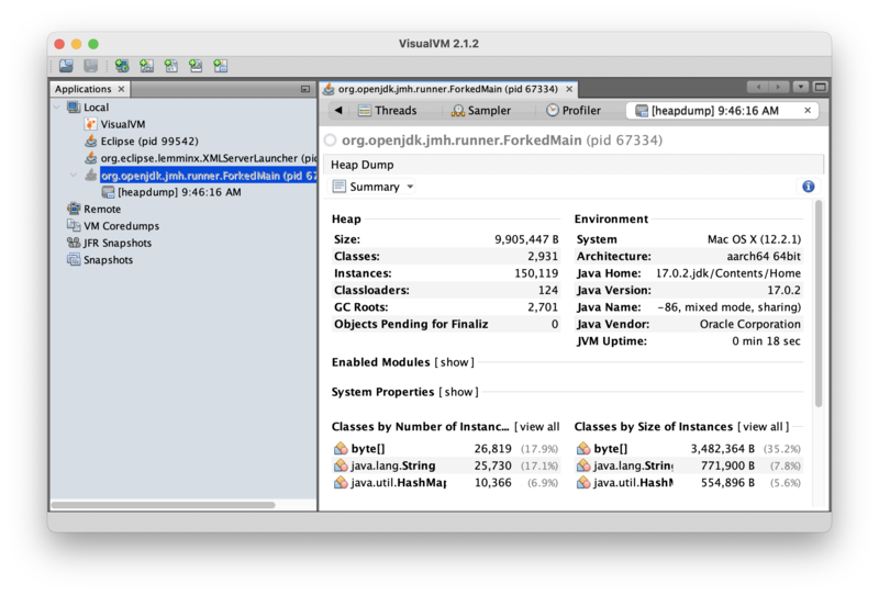
A heap dump is a snapshot of the live objects in the heap at the time of the dump. It’s an important tool for understanding application memory usage and allocation behavior. To investigate why Integer instances are being allocated, click the “Summary” pull-down box and select “Objects” to show the object browser, then type “Integer” in the Class Filter box to inspect Integer instances:

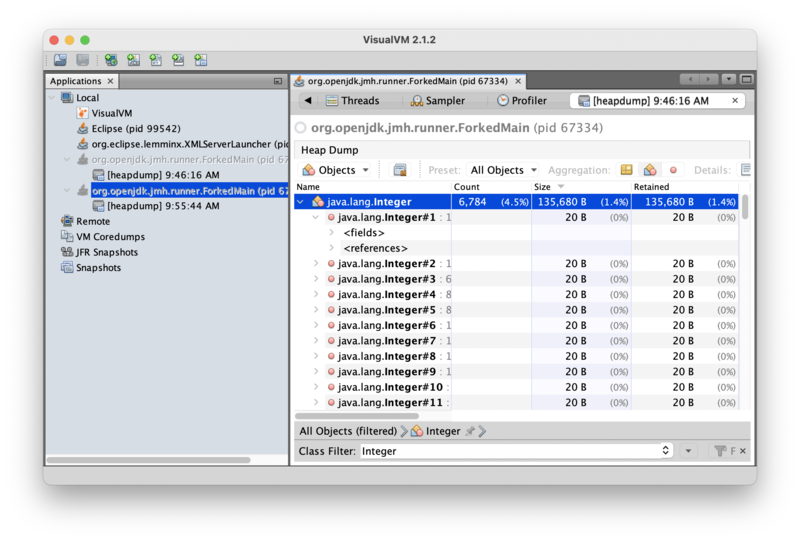
This view indicates that there are 6,784 live Integer objects in the heap, which is much less than just the 1.67M Integer objects allocated in the heap in real-time while the benchmark was in flight. This is an important clue: the Integer objects being allocated do not remain live for long, which increases confidence that the instances are allocated as part of text processing. Clicking on the “<references>” view of an instance will show the GC root referencing that instance:

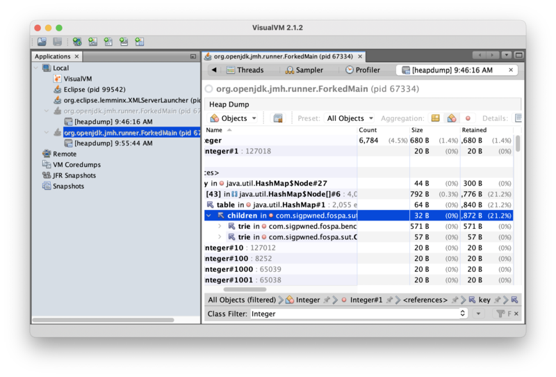
This particular Integer instance is a key in a HashMap. Continuing to drill into references shows the HashMap is part of DefaultGraphemeTrie, which holds the emoji processing data, and is in turn referenced by GraphemeMatcher. If the live Integer instances are part of DefaultGraphemeTrie, could the transient Integer instances allocated during text processing be related to DefaultGraphemeTrie, too?

The CPU profile indicated that most program time is spent in the GraphemeMatcher.find() method, so that seems like a reasonable place to start looking. The source code for that method is:

  public boolean find() {
    matched = false;
    start = end = -1;
    grapheme = null;

    while (index < length) {
      // Is there a grapheme starting at offset?
      int cp0 = text().codePointAt(index);
      int cc0 = Character.charCount(cp0);

      GraphemeTrie t = trie().getChild(cp0);
      if (t != null) {
        int offset = cc0;

        if (t.getGrapheme() != null) {
          matched = true;
          start = index;
          end = index + offset;
          grapheme = t.getGrapheme();
        }

        while (index + offset < length) {
          int cpi = text().codePointAt(index + offset);

          t = t.getChild(cpi);
          if (t == null)
            break;

          int cci = Character.charCount(cpi);

          offset = offset + cci;

          if (t.getGrapheme() != null) {
            matched = true;
            start = index;
            end = index + offset;
            grapheme = t.getGrapheme();
          }
        }

        if (matched()) {
          index = end;
          return true;
        }
      }

      index = index + cc0;
    }

    return false;
  }

This method calls the DefaultGraphemeTrie.getChild() method. The source code for that method is:

  private final Map<Integer, DefaultGraphemeTrie> children;
  private Grapheme grapheme;

  public DefaultGraphemeTrie() {
    this.children = new HashMap<>();
  }

  @Override
  public DefaultGraphemeTrie getChild(int codePoint) {
    return children.get(codePoint);
  }

Ah ha! The DefaultGraphemeTrie.getChild() method takes an int, and then calls Map.get(), which takes an object. Could the Integer instances be the result of autoboxing the primitive int into an Integer for the Map.get() call?

A direct way to test that theory would be to change the children variable from a Map<Integer,DefaultGraphemeTrie> to a primitive-friendly equivalent to avoid the autoboxing allocation. The fastutil library is an excellent collections library that includes primitive collections. Adding fastutil as a dependency and making the change results in the following updated workload code:

  private final Int2ObjectMap<DefaultGraphemeTrie> children;
  private Grapheme grapheme;

  public DefaultGraphemeTrie() {
    this.children = new Int2ObjectOpenHashMap<>();
  }

  @Override
  public DefaultGraphemeTrie getChild(int codePoint) {
    return children.get(codePoint);
  }

Rebuilding, re-running, and memory profiling the application confirms the theory! Integer instances are no longer allocated during processing:

And benchmark thread allocation is down from 760MB/sec to 5KB/sec (>99.9%):

Success!

Benchmarking the Change

Recall the following baseline benchmark results from Part I:

Benchmark                         Mode  Cnt   Score   Error  Units
GraphemeMatcherBenchmark.tweets                                thrpt   15       19.383 ±     0.482   ops/s
GraphemeMatcherBenchmark.tweets:·gc.alloc.rate                 thrpt   15       50.419 ±     1.252  MB/sec

In Part II, wall clock performance was optimized up to:

Benchmark                         Mode  Cnt   Score   Error  Units
GraphemeMatcherBenchmark.tweets                                thrpt   15       53.416 ±     2.194   ops/s

It’s time to re-run the benchmark again. (Remember to use the proper EC2 environment!) The performance results for the updated benchmark results follow here.

Result "com.sigpwned.fospa.benchmark.GraphemeMatcherBenchmark.tweets":
  46.292 ±(99.9%) 5.584 ops/s [Average]
  (min, avg, max) = (39.092, 46.292, 49.928), stdev = 5.223
  CI (99.9%): [40.709, 51.876] (assumes normal distribution)

Secondary result "com.sigpwned.fospa.benchmark.GraphemeMatcherBenchmark.tweets:·gc.alloc.rate":
  0.001 ±(99.9%) 0.001 MB/sec [Average]
  (min, avg, max) = (≈ 10⁻⁴, 0.001, 0.002), stdev = 0.001
  CI (99.9%): [≈ 0, 0.001] (assumes normal distribution)

So memory allocation got much better, but wall clock performance got worse.

Performance is a Balancing Act

This is an important lesson in performance analysis. In this post, the focus has been on reducing memory utilization, and certainly that was achieved: memory usage is down from roughly 50.419 MB/sec at baseline to much less than 1MB/sec. However, optimizing memory allocation has caused a wall clock performance regression of 13% from 53.416MB/sec to 46.292MB/sec.

In this way, performance analysis is like a game of whack-a-mole. An analyst focusing to optimize one dimension of performance can quickly find success, but in the process may cause other dimensions of performance to get worse, so optimization is often a tradeoff. Software optimization is not a zero-sum game, but not all dimensions of performance are correlated, either. It is frequently impossible to optimize all dimensions of performance at the same time; which dimension(s) to prioritize typically comes down to business value.

It’s unlikely that reducing memory allocation, and therefore GC work, reduced program wall-clock performance. The analyst could do another round of wall-clock optimization to see if performance can be improved in the low-allocation setting! Perhaps the performance drop is due to the performance of the new collection? In this way, performance analysis is an iterative practice. This is left as an exercise to the reader.

Next Steps

Now that memory allocation optimization is complete, we will wrap up this series in the conclusion. See you there!